Project Report, MAE 4150, University of Colorado Colorado Springs

Authors: Sean Glover, Matt Radel

Editors Note: That isn’t a typo, Colorado is included twice in the school name.

Abstract

Longswords are often treated as having static vibrational nodes, with implications for sparring. A combination of mathematical analysis, SolidWorks modeling, and practical experiments were used to analyze the motion of a longsword under realistic end conditions. It was determined that not only are the nodes not static with respect to different end conditions, they also vary over time during free vibration after an impulse. Due to the complexity of the vibrations, as well as the very specific design criteria of a sword, it is impractical to attempt to alter the sword to maintain specific node locations. Vibration damping gloves are suggested as a possible remedy to fatigue during sparring.

Nomenclature

w Displacement of blade [mm]

c Wave speed [m/s]

E Elastic modulus [Pa ]

a Acceleration of blade [m/s² ]

n Mode number [unitless]

τ tension [N]

ρ density [kg/m³]

v Velocity of blade [m/s]

L Blade length [m]

t Time after impact [sec]

x Linear distance along blade, measured from the hilt [m ]

Introduction

Longswords have a particularly long effective length. This, arising from the slender nature of a blade and the long blades used on such swords, makes them particularly vulnerable to vibrations. Vibrations are concerning for three principle reasons in a fencing context. First, vibrations transferred to the fencer through the hilt cause numbness and fatigue. Second, vibrations can prevent proper edge alignment. Third, energy going into a vibration is energy not going into the opponent, reducing the effectiveness of the strike.

Among contemporary longsword practitioners, there are several preconceived notions regarding vibrations that this study intends to examine for validity. The first and most common of these is the position of the vibrational node (commonly but incorrectly referred to as the center of percussion) near the end of the blade. This is commonly tested for by lightly gripping the hilt, often with just a finger and thumb, and slapping the pommel (the counterweight at the base of the grip) to provide an impulse and resulting vibrations. The sword will vibrate in a second mode, showing a clear node that is often around 10cm away from the tip. Conventional wisdom indicates that this is where a fencer should strike, as this will produce minimal vibrations. This also indicates second mode motion.

The second most common popular statement made about nodes refers to the positioning of the second node. A competent smith intends to place this at the point in the grip where the middle finger of the lead hand will mostly be positioned. The common test for this is similar to that performed for the other node, in that the grip is lightly held and an impulse to the pommel, moving where the grip is held until minimal vibration is felt in the hand.

These common tests and suggestions make a critical assumption: that the positions of the nodes do not change when the sword is held for actual sparring. This is a highly suspect assumption, as the end conditions of a vibrating beam have significant impact on the vibrational characteristics of the system. Determining the actual effects of hand position on vibrational nodes is the main purpose of this project. Additional information of interest is the actual amount of force lost to vibrations, as well as the force transferred to the hand of the fencer by vibration.

Model

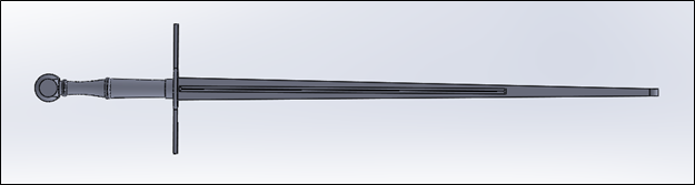
Two displacement tests were done using SolidWorks dynamic analysis. First, the sword was recreated as a SolidWorks CAD model, shown in Figure 1, as accurately as possible up to the bent tip. This tip was approximated as an elliptical ring at the end of the blade with similar dimensions as the true bend and is shown in Figure 2.

For the first displacement test, a small 0.057 cm² rectangle was cut out of the blade 85.39 cm up from the guard and a force of 250N was applied to that area for 0.02 seconds. The handle was then fixed on the upper and lower grips and a material of Plain Carbon Steel was applied to the entire sword (see Figure 2). These conditions were used to represent the sword getting struck by another, but no damping was assumed during the test.

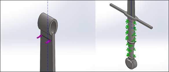
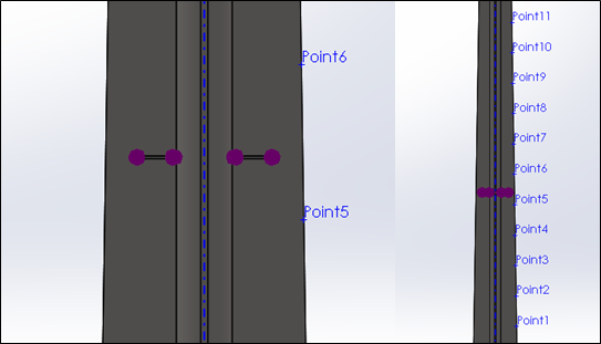
Figure 2:Rectangular force cut and sword tip (left) and fixed grip (right).

The second displacement test model had two small 0.0375 cm² rectangle cuts 15cm up from the guard and the same force was applied at these areas. There was only one fixed position on the upper grip and 30 points of interest were selected evenly distributed along the side of the blade (see Figure 3). Again, no damping was assumed during the test

Figure 3:Rectangular force cuts (left) and Distributed points of interest (right).

Solution

From the SolidWorks model, the second moments of area were calculated from the section 40cm away from the hilt, as a representative value for the blade:

Iz = 0.5089 cm⁴ = 5.089*10^-9m⁴
Iy = 0.0040 cm⁴= 4.0*10^-11m⁴

The stiffness of a beam is given by:

$K = \frac{3EIU}{L}$

The elastic modulus, E, for 51CrV4 Carbon Steel is variable based on the heat treatment. The specific heat treatment applicable here is not known. It is assumed the steel is tempered, for a value of 210GPa [1]. Therefore, the estimated stiffness for the sword is 3741 N/m in the blade direction and 29.40 N/m in the flat direction. This large difference between directions validates the assumption that the blade will experience negligible deflection, and therefore negligible vibration, around the blade’s axis. Another favorable feature is the thickness is consistent for most of the blade, and the width only decreases slightly, making the estimated second moment of area relatively accurate.

As the blade is most accurately thought of as a vibrating beam, it will be treated as a distributed-parameter system. The solution will be via the separation of variables method. The boundary conditions will be treated as cantilevered at the handle, and free at the tip. The handle itself will be treated as not vibrating, though this is a simplification.

The governing equation for the vibration of the blade is:

$w(x,t) = \sum_n a_n sin(\frac{n\pi c}{L}t) sin(\frac{n\pi}{L}) x$

Where n is the mode and the wave speed, c, is:

$c = \sqrt{\frac{E}{\rho}}$

As we are only dealing with the first two modes, n = 2. For this steel density of 7800 kg/m³ and elastic modulus of 210 GPa, c = 5188 m/s. Therefore, the equation of motion becomes:

$w(x,t) = a_1 sin(1902t) sin(3.666x) + a_2 sin(3804t)sin(7.332x)$

The constants are solved for via end conditions. The first end condition is w’’(0,0)=0. This is due to the assumption that there is no acceleration at the hilt at the beginning. For the second end condition, it will be assumed that the impulse provides an initial velocity to the tip, leading to w’(L,0)=20. This assumption is based on the only known data currently available regarding the speed of a sword [2]. From this test, the cutting surface moves at approximately 20m/s, making it a reasonable value for the resultant velocity from the impact. The initial displacement is 0. Therefore, solving for initial displacement provides no information. Taking the derivative of a multivariable function such as this simply entails taking the partial derivative with respect to each variable and adding the results. Therefore, the velocity equation is as follows:

$v(x,t)= 1902a_1 cos(1902t)sin(3.666x) + 3804a_2cos(3804t)sin(7.332x)+ 3.666a_1 sin(1902t)cos(3.666x)+7.332a_2sin(3804t)cos(7.332x)$

Solving for the velocity produces 1.2884a₂-0.3321a₁=20. From here, another derivative is needed for the acceleration condition:

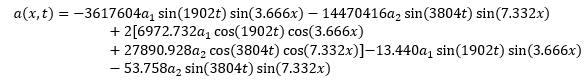
Editor’s Note: This is an image, because there is no way I’m converting this MS Equation to LaTeX

Solving for the acceleration condition produces a₁=-4a₄, allowing for the final constants to be determined and added to the initial equation:

$w(x,t) = -31.048sin(1902t)sin(3.666x)+7.762sin(3804t)sin(7.332x)$

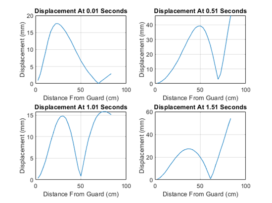
A graphical depiction of these results follows in Figure 4 and Figure 5:

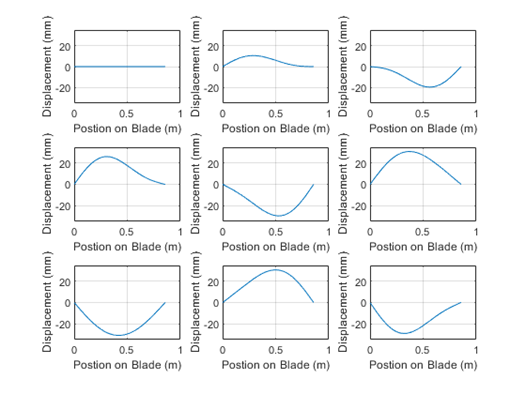
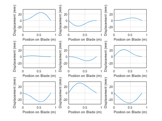
Figure 4: Time 0 to 1.6 (.2 sec between each graph)

Figure 5: Time 1.8 to 3.4 (.2 sec between each graph)

As can be seen in these graphs, there is no defined vibration node when the two modes are combined. As is to be expected with a multiple mode system, there is a fundamental frequency and a higher frequency harmonic of a lower amplitude.

Results

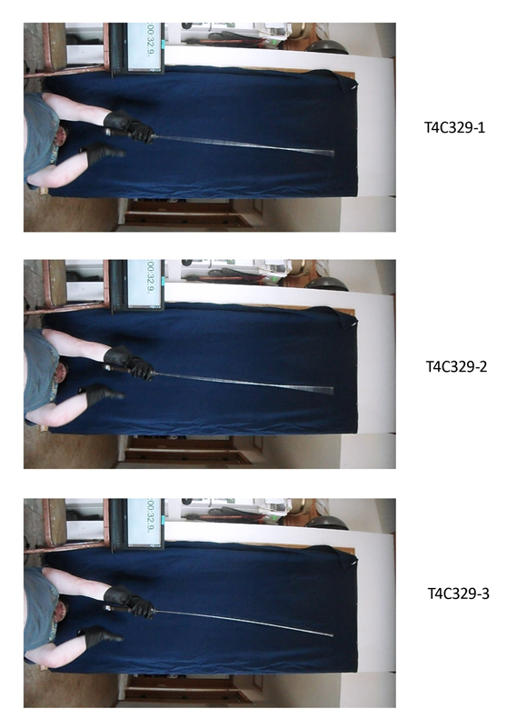
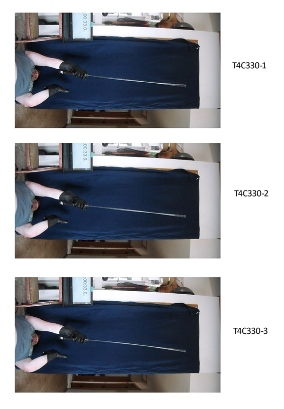
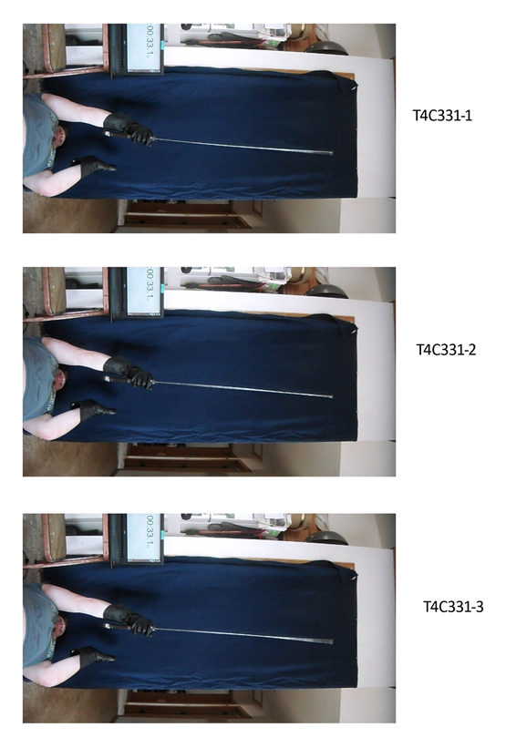
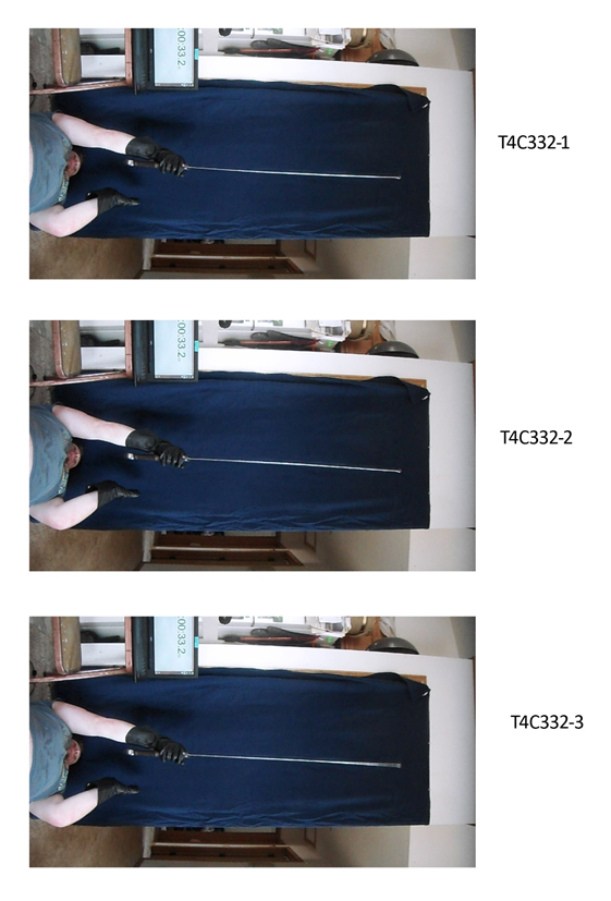
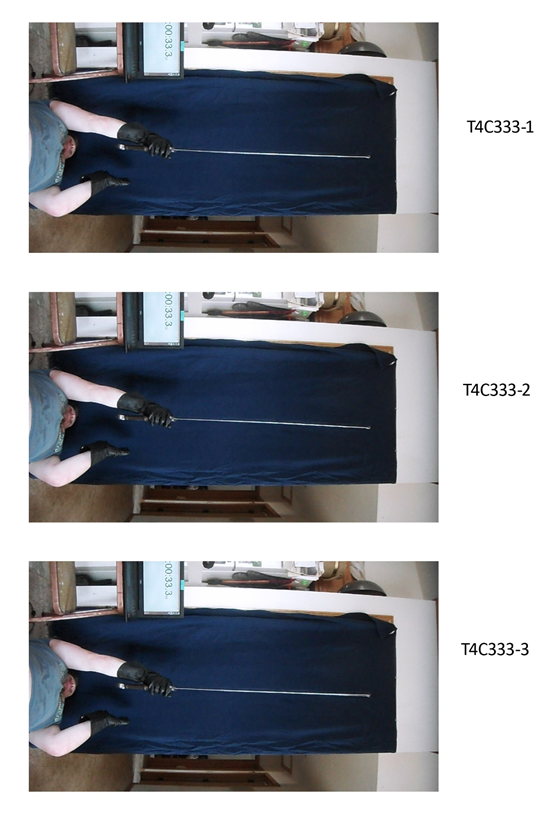
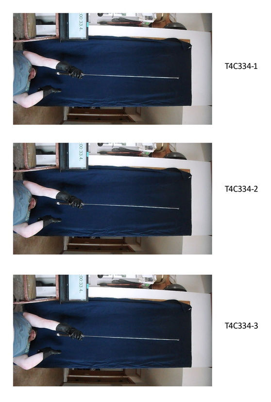
Practical tests in lieu of campus resources such as accelerometers required a certain amount of ingenuity. As clamped end conditions are not an accurate depiction of the realistic use conditions, tests were conducted in hand. To acquire useable data, a camera on a tripod was used in conjunction with a computer-based stopwatch to provide a stable reference time and position. At the start of testing videos, a grid with known dimensions was placed behind the sword to provide accurate scaling.

Tests were conducted with both one and two hands on the sword. For single-handed tests, the input was a tap with the hand to the pommel. A sample of frames from one of these tests can be found in appendix A. For two-handed tests, the original attempt was a strike with a wooden mallet, but it provided insufficient vibration. After some experimenting with different surfaces, it was found the most effective input is an elastic material with some give. The final tests in this manner used an input of bouncing the blade off a large exercise ball. Given the inherent limits of the equipment at hand, accurate data regarding the input force is unavailable. Unfortunately, this means the force transmissibility was impossible to experimentally verify. In addition, the position of the second vibrational node was also not able to be determined by this method.

After testing, videos were examined in Photoshop to determine amplitudes and vibrational node positions. Difference analysis between frames allowed for depiction of the full amplitude in a single image. This analysis can be found in Figure 6:

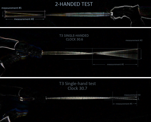
Figure 6: Difference analysis of 2 tests.

The measurements from these tests are given in Table 1:

Test	Amplitude (cm)	Node position from tip (cm)
2-handed test	5.13	36.41
1-handed test at clock time 30.6	11.63	49.36
1-handed test at clock time 30.7	3.25	27.15

This is interesting, as it experimentally verifies that the node location not only changes based on hand position, but it also changes in a very short period within the same test, with essentially identical conditions. A difference of more than 20cm across a tenth of a second indicates that the vibration is much more complex than previously thought. The assumption that the node is essentially static is now shown to be incorrect not only for other hand positions, but for different points in time during the same vibrational response to an impact! This also agrees well with the results of the mathematical model.

Determining the single-hand frequency posed a challenge. The vibration was easily visible in the videos, but the frequency was near enough to the frame rate that Nyquist Frequency effects were a possible concern. From visual analysis of the vibration, the frequency was estimated at around 10-20 Hz. Given a frame rate of 30fps, this was concerning, as any vibration above 15 Hz would be impossible to accurately measure via video analysis.

Analysis of the video suggests a frequency of approximately 10 Hz. However, the vibrations visible in the frames are complex and difficult to determine. Difficulty determining the frequency in this manner means the natural frequency of the single hand case cannot be experimentally verified with confidence, given available equipment.

While the single-hand frequency was a large enough amplitude and low enough frequency to detect in the video, the two-hand frequency was much higher. This necessitated a different test method. Audio was taken of the blade being impacted. This audio was analyzed via Spectrum Lab FFT analysis software. The natural frequency was faintly visible, occurring at 1233.9 Hz. Spek frequency analysis software provided a less measurable but more visible example of this analysis, found in Figure 7:

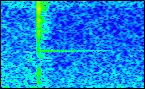
The entire test raster can be found with commentary in appendix B. As a distributed parameter system such as this has a fundamental natural frequency and multiple harmonics, this is presumably not the only frequency of interest. However, it was the only frequency detectable with the available equipment.

This frequency can be converted to 7752.82 radians per second. The theoretical model of the sword suggests a fundamental frequency of 1902 radians per second. This could indicate a significant flaw with the model. However, the measured frequency is approximately 4.08 times the calculated one. This, assuming some level of imprecision with the assumptions made in the mathematical model, suggests the measured frequency is a harmonic of the fundamental frequency. It was near the edge of the microphone’s lower range and was relatively low amplitude. As harmonic frequencies have lower amplitudes than the fundamental frequency, the next higher harmonic was likely below the noise floor. This also supports the notion that the calculated fundamental frequency is accurate.

SolidWorks Simulation Results

The first displacement test gave a response corresponding closely, each off by a factor of about 300 when the force was applied, to the first mode of motion shown in appendix E. The only node found using this test was located at the handle. This was expected for the used end conditions of the blade and placement of the force. The maximum displacement for the points of interest occurred 83.4 cm from the guard and the displacement became smaller as the distance from the grip decreased.

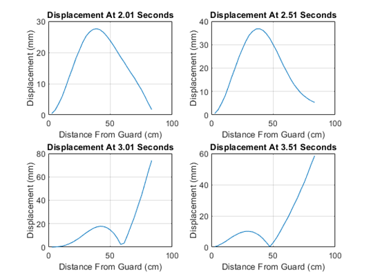
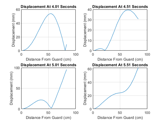
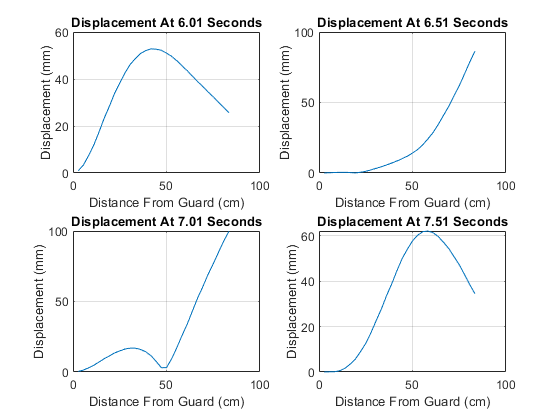
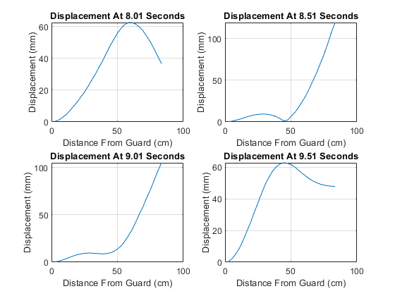
The second displacement test gave more variable results for the nodes. The nodes were not stationary along the blade and instead moved over time. The main locations of the nodes were near points 1, 7, 17, 21, 25, and 30 which correspond to 84.72cm, 68.04cm, 45.8cm, 29.12cm, 18cm, and 4.1cm from the tip of the blade, respectively.

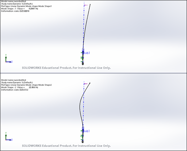
These shifting nodes suggest that the vibrations in the sword are made through an overlapping of multiple modes. The first five modes are shown in appendix E, were calculated using SolidWorks vibration analysis, and occur with frequencies of 4.0426 Hz, 20.978 Hz, 50.253 Hz, 56.636 Hz, and 109.82 Hz. The first two modes are shown in Figure 8. These time dependent nodes correlate with the experimental tests done with the real sword.

Figure 8: Modes 1 (top) and 2 (bottom) of the sword.

Modifications

Modifying swords is a difficult prospect if the sword is to remain useful afterward. The balance, blade cross-section, length, and grip all have many design constraints more important than vibration suppression. For instance, addition of a vibrational absorber such as attached to power lines would obviously be unsuitable for the middle of a longsword’s blade. As the most common sources of vibration are the impulses of hitting either an opponent or an opponent’s blade, limiting the input or adding dampers are likewise not valid options. Two possibilities seem immediately obvious. The grip could be modified to attempt to decrease vibration, or the fencer could adjust their hands to produce favorable vibrational characteristics via tuning of the end conditions.

The first option is the most straightforward, and the most achievable. Either the grip could be wrapped in a damping layer, such as a polymer foam, or sparring gauntlets could incorporate vibration damping in a similar manner. This has two drawbacks. First, it reduces the tactile feedback from the grip, which is valuable information for the fencer. Second, it only mitigates transmissibility to the fencer. It produces no significant effect regarding the location of a vibrational node, nor will it prevent vibrations in the blade causing edge misalignment or reduced force.

The second option relies on being able to maintain very specific end conditions in a complex and stressful situation. This may be possible with training; however difficult it may be. Such a method would allow an experienced fencer to intentionally strike with the vibrational node for the best effect. Combining this with damping at the grip could potentially allow for better performance during sparring. However, as the node positions change more than was originally thought, far more testing would be required before this could be a feasible option. Additionally, such complex requirements would likely interfere with other aspects of sparring.

Conclusion

The vibrational characteristics of longswords are far more complex than previously believed. Not only do the vibrational nodes move positions based on different end conditions, they also change position during vibrations from an impact. This indicates there are multiple modes at play. Without accelerometers it would be extremely difficult to fully characterize these vibrations. Even upon characterizing these vibrations, it would be extremely difficult to alter the design of a sword to isolate, damp, or otherwise tune the vibrations to a specific purpose. As vibrations transmitted into the hand are fatiguing to fencers, it is possible vibration damping materials such as polymer foams would help mitigate this issue.

It bears noting that the design of many swords, including the one tested here, includes a fuller. This is the groove cut down the middle of the flat of the blade on both sides, and it functions in the same manner as the design of an I-beam. It increases stiffness, which decreases the amplitude of vibrations. In this manner, it could be claimed the sword is already designed to mitigate vibration, in a manner consistent with its application. Many different fuller designs are possible, and it would merit further study of these designs to determine which fullers produce the most favorable result. That is, however, beyond the scope of this paper.

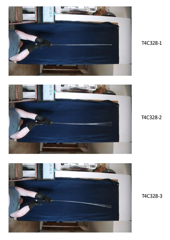
Appendix A: Sequence of test video frames

In the following images, the final numbers indicate the time of the frame. As the video sampled at 30fps, every tenth of a second had 3 associated frames. The last number is the frame within each tenth of a second.

Appendix B: Two-handed natural frequency spectrum and commentary

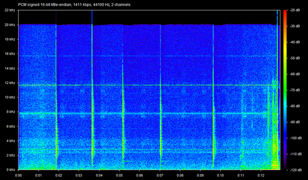
The test had 5 impacts on the sword, shown in the broadband, short duration signals visible. The natural frequency had been previously estimated via matching to test tones as being around 1kHz. The third and fourth tests had sufficient ringing to be detected by the microphone, shown as the longer duration pure tones near 1kHz, as expected. This was then measured with greater detail in Spectrum Lab, providing the natural frequency.

Appendix C: Sword Displacement Tables

distance (cm) from tip	distance(cm) From guard	Time(s) and Point Displacement (mm)
distance (cm) from tip	distance(cm) From guard	.01sec	.51sec	1.01sec	1.51sec	2.01sec	2.51sec	3.01sec
84.72	2.78	0.910	0.242	0.347	0.516	0.459	0.644	0.025
81.94	5.56	3.000	0.870	1.220	1.800	1.610	2.250	0.132
79.16	8.34	6.200	2.010	2.720	3.990	3.600	5.020	0.415
76.38	11.12	9.300	3.370	4.400	6.440	5.870	8.130	0.866
73.60	13.90	12.600	5.260	6.560	9.570	8.820	12.200	1.660
70.82	16.68	15.200	7.500	8.810	12.900	12.000	16.500	2.800
68.04	19.46	16.700	9.770	10.700	15.800	14.900	20.400	4.130
65.26	22.24	17.600	12.600	12.600	18.900	18.100	24.600	5.950
62.48	25.02	17.600	15.400	13.900	21.400	20.700	28.100	7.810
59.70	27.80	17.100	18.800	14.700	23.800	23.300	31.400	10.100
56.92	30.58	16.200	22.500	14.800	25.600	25.300	34.100	12.300
54.14	33.36	15.200	25.800	14.300	26.700	26.600	35.700	14.200
51.36	36.14	13.900	29.500	12.900	27.300	27.400	36.700	16.000
48.58	38.92	12.600	32.500	11.100	27.200	27.600	36.800	17.200
45.80	41.70	11.100	35.600	8.500	26.400	27.300	36.100	17.800
43.02	44.48	9.530	37.800	5.460	24.800	26.400	34.600	17.600
40.24	47.26	8.150	39.000	2.550	22.800	25.200	32.600	16.600
37.46	50.04	6.680	39.200	0.847	19.700	23.700	29.900	14.600
34.68	52.82	5.510	38.100	3.760	16.300	22.100	27.200	11.800
31.90	55.60	4.330	35.400	6.800	11.700	20.300	24.000	7.640
29.12	58.38	3.280	31.000	9.420	6.260	18.500	20.900	2.360
26.34	61.16	2.430	25.700	11.300	0.875	16.900	18.200	3.310
23.56	63.94	1.520	18.700	13.100	5.760	15.100	15.400	10.400
20.78	66.72	0.673	10.700	14.400	12.700	13.400	13.000	18.200
18.00	69.50	0.039	2.940	15.200	19.000	11.800	11.100	25.800
15.22	72.28	0.691	6.580	15.700	26.300	9.910	9.300	35.000
12.44	75.06	1.230	15.500	15.800	32.800	8.130	8.030	43.600
9.66	77.84	1.800	25.900	15.800	40.200	6.010	6.900	53.800
6.88	80.62	2.380	36.600	15.500	47.600	3.770	6.020	64.400
4.10	83.40	2.910	46.300	15.100	54.100	1.710	5.370	74.000

*Bold Values correspond to lowest recorded value at that time

distance (cm) from tip	distance(cm) From guard	Time(s) and Point Displacement (mm)
distance (cm) from tip	distance(cm) From guard	3.51sec	4.01sec	4.51sec	5.01sec	5.51sec	6.01sec	6.51sec
84.72	2.78	0.292	0.209	0.226	0.292	0.360	0.975	0.060
81.94	5.56	0.999	0.791	0.705	1.050	1.240	3.370	0.186
79.16	8.34	2.170	1.920	1.340	2.410	2.720	7.410	0.349
76.38	11.12	3.420	3.360	1.820	4.030	4.350	11.900	0.460
73.60	13.90	4.940	5.500	2.060	6.220	6.390	17.400	0.483
70.82	16.68	6.450	8.190	1.830	8.710	8.550	23.300	0.339
68.04	19.46	7.680	11.000	1.110	11.100	10.500	28.400	0.041
65.26	22.24	8.850	14.700	0.324	13.800	12.600	33.900	0.529
62.48	25.02	9.620	18.200	2.130	16.100	14.400	38.300	1.220
59.70	27.80	10.100	22.600	4.750	18.400	16.400	42.600	2.190
56.92	30.58	10.100	27.100	7.900	20.300	18.100	46.200	3.330
54.14	33.36	9.720	31.200	11.000	21.400	19.600	48.700	4.440
51.36	36.14	8.750	35.800	14.800	21.900	20.900	50.900	5.780
48.58	38.92	7.420	39.700	18.300	21.600	21.900	52.100	7.040
45.80	41.70	5.410	43.900	22.200	20.300	22.800	52.800	8.550
43.02	44.48	2.910	47.600	26.000	17.900	23.400	52.700	10.200
40.24	47.26	0.339	50.300	29.100	14.800	23.800	52.200	11.900
37.46	50.04	3.000	52.600	32.300	10.100	24.100	51.000	14.200
34.68	52.82	6.200	53.700	34.700	4.870	24.500	49.600	16.700
31.90	55.60	10.000	53.700	36.800	2.110	25.200	47.700	20.200
29.12	58.38	14.100	52.200	38.300	10.100	26.300	45.500	24.400
26.34	61.16	18.000	49.500	39.100	18.000	27.900	43.500	29.000
23.56	63.94	22.400	45.200	39.400	27.400	30.200	41.100	34.800
20.78	66.72	27.100	39.700	39.300	37.200	33.100	38.800	41.200
18.00	69.50	31.500	33.900	38.800	46.100	36.400	36.700	47.500
15.22	72.28	36.700	26.200	37.700	56.400	40.700	34.400	55.000
12.44	75.06	41.500	18.700	36.500	65.600	45.100	32.400	62.000
9.66	77.84	47.200	9.470	34.700	76.000	50.500	30.100	70.300
6.88	80.62	53.100	0.573	32.600	86.400	56.400	27.800	78.700
4.10	83.40	58.500	9.170	30.700	95.600	61.800	25.700	86.400

*Bold Values correspond to lowest recorded value at that time

distance (cm) from tip	distance(cm) From guard	Time(s) and Point Displacement (mm)
distance (cm) from tip	distance(cm) From guard	7.01sec	7.51sec	8.01sec	8.51sec	9.01sec	9.51sec	9.96sec
84.72	2.78	0.392	0.053	0.350	0.281	0.317	0.667	0.178
81.94	5.56	1.360	0.082	1.240	0.959	1.080	2.390	0.595
79.16	8.34	3.000	0.094	2.800	2.080	2.320	5.470	1.250
76.38	11.12	4.800	0.584	4.610	3.270	3.630	9.110	1.890
73.60	13.90	7.070	1.670	7.040	4.710	5.190	14.100	2.570
70.82	16.68	9.420	3.460	9.800	6.130	6.670	19.700	3.050
68.04	19.46	11.400	5.700	12.500	7.280	7.810	25.200	3.210
65.26	22.24	13.500	9.000	15.700	8.350	8.790	31.600	2.980
62.48	25.02	15.000	12.600	18.800	9.030	9.350	37.400	2.320
59.70	27.80	16.300	17.300	22.500	9.430	9.610	43.600	1.040
56.92	30.58	16.900	22.600	26.500	9.370	9.540	49.200	0.807
54.14	33.36	16.900	27.700	30.200	8.870	9.290	53.600	2.830
51.36	36.14	16.000	33.600	34.600	7.790	8.980	57.600	5.410
48.58	38.92	14.300	38.800	38.700	6.310	8.840	60.200	7.800
45.80	41.70	11.500	44.600	43.400	4.050	9.050	62.000	10.400
43.02	44.48	7.520	49.900	48.000	1.110	9.890	62.700	12.600
40.24	47.26	3.020	54.000	52.000	2.140	11.300	62.500	14.000
37.46	50.04	3.160	57.700	56.000	6.490	13.900	61.500	14.900
34.68	52.82	9.490	60.200	59.000	11.100	17.200	60.100	14.800
31.90	55.60	17.500	61.700	61.400	17.000	22.100	58.100	13.800
29.12	58.38	26.100	62.000	62.600	24.000	28.100	56.100	11.700
26.34	61.16	34.200	61.200	62.600	31.200	34.500	54.400	8.970
23.56	63.94	43.500	59.400	61.600	40.000	42.500	52.600	5.330
20.78	66.72	52.700	56.900	59.700	49.600	51.000	51.200	1.220
18.00	69.50	60.700	54.200	57.300	58.900	59.000	50.100	2.800
15.22	72.28	69.400	50.600	53.800	70.200	68.300	49.200	7.520
12.44	75.06	76.900	47.100	50.300	80.800	76.800	48.600	11.900
9.66	77.84	85.000	42.800	45.900	93.500	86.500	48.200	16.900
6.88	80.62	92.900	38.400	41.200	107.000	96.400	47.900	21.900
4.10	83.40	99.800	34.400	36.800	119.000	105.000	47.800	26.400

*Bold Values correspond to lowest recorded value at that time

Appendix D: Point Displacement Graphs

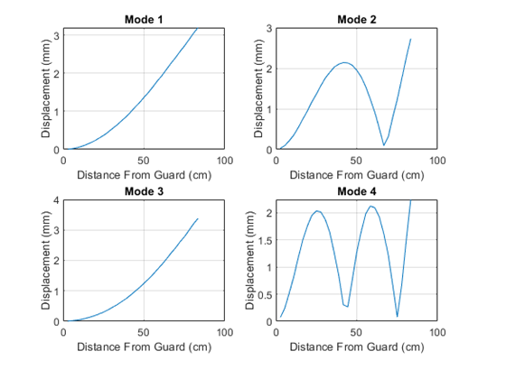
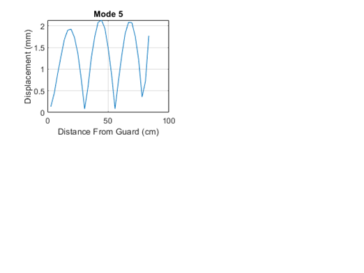
Appendix E: Mode Displacement Table and Graphs

Distance (cm) from tip	Distance(cm) From guard	Displacement (mm)
Distance (cm) from tip	Distance(cm) From guard	Mode 1 4.0426 Hz	Mode 2 20.978 Hz	Mode 3 50.253 Hz	Mode 4 56.636 Hz	Mode 5 109.82 Hz
84.72	2.78	0.004989	0.027100	0.007610	0.072300	0.135000
81.94	5.56	0.018310	0.095900	0.018700	0.246000	0.437000
79.16	8.34	0.043150	0.217000	0.038100	0.528000	0.884000
76.38	11.12	0.073780	0.356000	0.062000	0.826000	1.290000
73.60	13.90	0.117600	0.542000	0.096500	1.180000	1.680000
70.82	16.68	0.171200	0.750000	0.139000	1.500000	1.900000
68.04	19.46	0.226600	0.945000	0.184000	1.750000	1.920000
65.26	22.24	0.297700	1.170000	0.243000	1.950000	1.730000
62.48	25.02	0.368200	1.360000	0.303000	2.030000	1.360000
59.70	27.80	0.455700	1.570000	0.378000	2.010000	0.777000
56.92	30.58	0.551300	1.760000	0.462000	1.870000	0.080900
54.14	33.36	0.642900	1.900000	0.544000	1.630000	0.585000
51.36	36.14	0.753000	2.030000	0.645000	1.250000	1.270000
48.58	38.92	0.856900	2.100000	0.742000	0.834000	1.750000
45.80	41.70	0.980200	2.140000	0.860000	0.303000	2.080000
43.02	44.48	1.110000	2.130000	0.987000	0.266000	2.130000
40.24	47.26	1.230000	2.070000	1.110000	0.764000	1.940000
37.46	50.04	1.371000	1.950000	1.250000	1.280000	1.470000
34.68	52.82	1.500000	1.780000	1.390000	1.660000	0.864000
31.90	55.60	1.650000	1.540000	1.540000	1.980000	0.083400
29.12	58.38	1.804000	1.240000	1.710000	2.120000	0.721000
26.34	61.16	1.944000	0.915000	1.870000	2.090000	1.320000
23.56	63.94	2.104000	0.520000	2.050000	1.920000	1.820000
20.78	66.72	2.266000	0.093300	2.240000	1.610000	2.080000
18.00	69.50	2.410000	0.315000	2.410000	1.220000	2.070000
15.22	72.28	2.574000	0.793000	2.610000	0.661000	1.750000
12.44	75.06	2.721000	1.230000	2.780000	0.078500	1.210000
9.66	77.84	2.886000	1.740000	2.990000	0.679000	0.357000
6.88	80.62	3.052000	2.260000	3.200000	1.490000	0.715000
4.10	83.40	3.200000	2.730000	3.380000	2.240000	1.770000

*Bold Values correspond to node points.